6.3. Control the Cluster Shape

Tip

The sample input and output files can be found in testfiles/geom/1-shape.

In this Section we will introduce how to use components block to accurately control the cluster shape. You will see how powerful geom is.

6.3.1. General Input

In this section we will use the same input for all examples, only changing the lm_dir and components block.

geom.inp

lm_dir          TODO     # Save the local minima to this folder.
num_calcs       10       # Total number of calculations.
do_coarse_opt   yes      # no: Do NOT the coarse optimization.
min_energy_gap  1.E-4    # When two energies differ smaller than
                         # this value, they are treated as identical.
                         # A negative number means do not remove
                         # energetically degenerated ones.
max_geom_iters  3000     # The maximum number of iterations for local optimization.
                         # If it is less or equal than zero, then the number is unlimited.

components
  TODO
end

commands
end

You can see that, compared with the one given in Input File for geom, the charmm, xtb, and savegjf are deleted, since we do not need them. Also, the commands block is left empty, since we do not need any third party programs. We just use geom as a structure generator. For each system, we generate only 10 clusters, as indicated by num_calcs.

6.3.2. Example: box, (C6H6)512(H2O)2048

We will consider the cluster of 512 \(\mathrm{C}_6\mathrm{H}_6\) and 2048 \(\mathrm{H}_2\mathrm{O}\). First we prepare their structure:

c6h6.xyz

12
C6H6
C                  0.00000000    1.39649000    0.00000000
C                  1.20939600    0.69824500    0.00000000
C                  1.20939600   -0.69824500    0.00000000
C                  0.00000000   -1.39649000    0.00000000
C                 -1.20939600   -0.69824500    0.00000000
C                 -1.20939600    0.69824500    0.00000000
H                  0.00000000    2.48319100    0.00000000
H                  2.15050600    1.24159500    0.00000000
H                  2.15050600   -1.24159500    0.00000000
H                  0.00000000   -2.48319100    0.00000000
H                 -2.15050600   -1.24159500    0.00000000
H                 -2.15050600    1.24159500    0.00000000

h2o.xyz

3
water
O                  0.00000000    0.00000000   -0.11081188
H                  0.00000000   -0.78397589    0.44324751
H                 -0.00000000    0.78397589    0.44324751

6.3.2.1. Mixture

First, we want to get a solvent box of their mixture. Here, the keyword box will be used. In h2o-c6h6-mixture.inp, change the component block:

h2o-c6h6-mixture.xyz

lm_dir  h2o-c6h6-mixture
components
    c6h6.xyz 512
    box 0 0 0 45 90 45
    ****
    h2o.xyz 2048
    box 0 0 0 45 90 45
    ****
end

Here we can see that：

Each component is separated by ****;
The first line of each component is the structure file name (path can be included) and its number. Say h2o.xyz 2048 means that there are 2048 water, whose structure is defined in h2o.xyz.
The second line of each component is its shape of packing.

In this case, both components have the shape box:

Note

box x0 y0 z0 x1 y1 z1

Uniformly distribute molecules in a box determined by (x0, y0, z0) and (x1, y1, z1).

Since \(\mathrm{C}_6\mathrm{H}_6\) and \(\mathrm{H}_2\mathrm{O}\) are distributed in the same space, they will form a perfect mixture.

Now run the program:

$ geom h2o-c6h6-mixture.inp > h2o-c6h6-mixture.out

6.3.2.2. Bi-phase

Since \(\mathrm{C}_6\mathrm{H}_6\) and \(\mathrm{H}_2\mathrm{O}\) do not solvate each other, it is possible to generate a bi-phase cluster. Just let them distribute in different but adjoint boxes!

h2o-c6h6-biphase.xyz

lm_dir  h2o-c6h6-biphase
components
    c6h6.xyz 512
    box 0 0 0 45 45 45
    ****
    h2o.xyz 2048
    box 0 45 0 45 90 45
    ****
end

Now run the program:

$ geom h2o-c6h6-biphase.inp > h2o-c6h6-biphase.out

Now, let us compare the structures. Just randomly take 2, say h2o-c6h6-mixture/3.xyz and h2o-c6h6-biphase/2.xyz. See below, we perfectly get what we want!

6.3.3. Example: random, (H2O)50

There is a keyword random that is very similar to box:

Note

random x0 y0 z0 x1 y1 z1

Randomly distribute molecules in a region determined by (x0, y0, z0) and (x1, y1, z1).

Unlike box, which tend to put molecules uniformly, random will put molecules randomly. Let’s try it for 50 water molecules.

h2o50.xyz

lm_dir  h2o50
components
    h2o.xyz 50
    random 0 0 0 15 15 15
    ****
end

Now run the program:

$ geom h2o50.inp > h2o50.out

One structure, say h2o50/3.xyz, is shown below. We compared it with a structure generated by replacing random to box.

6.3.4. Example: fix, H2O in SSZ-13

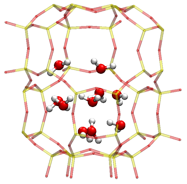
We want to study the diffusion of \(\text{H}_2\text{O}\) in zeolite SSZ-13. The structure of SSZ-13 is given below:

ssz-13.xyz

108
SSZ-13
  O         5.7000232468        7.6303196339        2.6186286767
  O         5.2045498989       10.1995252965        3.2272552812
  O         7.6341828896        9.4099723840        2.7745789292
  O         5.8753034436        9.5497196844        0.7672162010
  O         7.6375473635        4.2759815544        2.6753670218
  O         9.5707533006        7.6299616532        2.6176480074
  O         9.6106668261        5.3414448452       13.6228779840
  O         7.6185326402        8.7535796994       13.6836873966
  O         5.6658146587        5.3461814248       13.6160993667
  O         5.7026893239       -0.2642085908        7.5407946669
  O         0.7825962064        8.1512328930        7.5378038833
  O         2.7836661828       11.6286830319        7.5359961843
  O         2.7363955771        9.3420684719        3.8535391861
  O         7.6423184053        0.8505970745        3.7730132707
  O        12.5335364638        9.3415768142        3.8544585628
  O        12.4624155643        3.6818551888       12.4626958554
  O         7.6062858624       12.1072824025       12.4587051589
  O         2.8065149113        3.6894351696       12.2320710199
  O         2.7322963802        1.4435907562        8.8508132419
  O         0.8127191930        4.8681935127        8.6967338458
  O        12.4822455137        1.3976417344        8.7679437480
  O         5.6527918209        2.5629377561        3.2319866240
  O        12.0423876809        6.7757052402        3.2233313473
  O        12.0554980341        6.2591391560       13.0723873245
  O         5.5916803863       10.4417381114       13.0790389503
  O         5.1667070765        2.7598543540       13.1500955201
  O        10.0234139879        2.7573797734       13.0802094325
  O         9.6173269693       10.4509455156       13.0839569435
  O         3.1861034312        6.1951039344       13.1391153838
  O         3.2262073712        6.7771124228        3.2237580685
  O         9.6209190582        2.5656089905        3.2277416465
  O        10.0640705757       10.1974856514        3.2288444611
  O         5.1427255382        2.3096527675        8.0673522413
  O        12.4246061731        6.5049032168        8.1596286214
  O         5.2287254916       10.6584161272        8.1499333643
  O        10.0660760251       10.7260767207        8.1486535093
  O         2.8490782073        6.5139838953        8.1476193260
  O        10.0374817601        2.3659377558        8.1472483774
  O         5.1316112190        5.0641064531        2.8432015310
  O        10.1446584873        5.0657040841        2.7757616149
  O        10.1029249905        7.9248177185       13.5271012901
  O         5.1139616931        7.9307810948       13.5327555244
  O         7.6221919820        3.6097600857       13.5295025529
  O         7.6288414056        1.5118665409        7.7615136197
  O        11.9654721427        9.0151964046        7.6848839357
  O         3.2451981211        9.0440458535        7.6881718795
  O         3.3069973094       11.9100887748        3.6976804332
  O         5.1307773743        0.0649280529        3.6340011283
  O         0.7969499830        7.5670851250        3.6935855226
  O         0.7910818700        5.3346368625       12.6820331150
  O        11.9636291062        1.1105277839       12.6111708865
  O         3.2392803629        1.1213561083       12.5479345449
  O         3.3075057508        4.0157430778        8.7760041016
  O        12.0156624591        3.9738388657        8.6139906116
  O         7.6320672727       11.5168215978        8.6125370060
  O         5.8866593170        3.4930627815        0.7891245303
  O        11.1355336190        6.5074683788        0.7610373808
  O         9.3801650379        3.4821683317        0.7717307825
  O         9.3883869933        9.5474036098        0.7666774122
  O         4.1692472661        6.4488991333        0.7780060769
  O         5.9556046254        1.6428018426        5.6765493427
  O        12.6861939240        7.3729754052        5.6887347990
  O         4.3586450055       10.4595476971        5.6921261702
  O         2.5801899718        7.3759353889        5.6905185401
  O         9.3400531831        1.7041165806        5.6889457138
  O        10.9432024258       10.5171940688        5.6851549584
  O        12.7365486472        5.5973335861       10.6155686479
  O         5.8478045129       11.3130579735       10.6124834850
  O         4.5150336200        2.4391618565       10.6065434296
  O         9.3801870229       11.2550644389       10.6124530044
  O         2.4362265224        5.7858392934       10.6232169362
  O        10.9023169714        2.5612785425       10.6093785249
 Si         6.0920814665        3.8508163034        2.3648358150
 Si        10.7202283849        6.5092425635        2.3328070616
 Si        10.7198656965        6.4925660943       13.9546031759
 Si         6.0652860896        9.1709124986       13.9647009255
 Si         6.0809445096        3.8112454238       13.9744263842
 Si         9.1680499571        3.8090892108       13.9600924915
 Si         9.1702883031        9.1714808622       13.9670464697
 Si         4.5450589507        6.4778439590       13.9665556825
 Si         4.5589301028        6.4970522597        2.3544741665
 Si         9.1776796571        3.8440220779        2.3459143784
 Si         9.1743108787        9.1858945424        2.3361918038
 Si         6.1023939667        1.2912554713        7.2563853198
 Si        12.8984444715        7.7609462493        7.2559239768
 Si         3.8937893347       10.4628352540        7.2542014120
 Si         3.8917972712       10.4639571217        4.1313484718
 Si         6.1021660505        1.2768708902        4.0983248150
 Si        12.9264443751        7.7793779850        4.1294213351
 Si         2.3418034349        7.7806749736        4.1302867232
 Si         9.1747023738        1.2939288098        4.1186514298
 Si        11.3852128233       10.4740999990        4.1168223128
 Si        11.3849847412       10.4645367999        7.2520286806
 Si         2.3463927644        7.7693527709        7.2545905923
 Si         9.1641901801        1.3288002236        7.2655864551
 Si        12.9252078158        5.2179055842       12.1892578243
 Si         6.0541114995       11.7025286295       12.1775311953
 Si        12.9318493098        5.2383696707        9.0377621396
 Si         6.0833435431       11.6953330771        9.0489768990
 Si         9.1739017270       11.7144997047        9.0639602124
 Si         2.3459232172        5.2847394268        9.0735577386
 Si        11.3678806369        2.5575039972        9.0491343651
 Si        11.3433313927        2.5385553857       12.1747149889
 Si         9.1561829214       11.6952711342       12.1629072761
 Si         2.3228901646        5.2436972032       12.1586452445
 Si         6.0937069986        9.1867058586        2.3360857945
 Si         3.9151902179        2.5466565165        9.0895664436
 Si         3.9346333440        2.5195603195       12.1307588181

In this case, SSZ-13 should be fixed in space, and water molecules are put into its big cage. In this case, a new keyword fix will help:

Note

fix x y z

Put the center of the molecule at (x, y, z), with a random rotation.

fix x y z alpha beta gamma

Put the center of the molecule at (x, y, z), with a rotation (alpha, beta, gamma). So, fix x y z 0 0 0 will not rotate the molecule but keep it orientation as in its XYZ file.

We fix the center of SSZ-13 at (0, 0, 0) without any rotations, so:

h2o-ssz-13.inp

lm_dir  h2o-ssz-13
components
    ssz-13.xyz 1
    fix 0 0 0 0 0 0
    ****
end

After running the optimization, you will find that SSZ-13 have been moved that its center is at the origin without rotations. Now we can try to determine a box inside the cage to let us put water in.

Tip

Their are a lot of ways to do this. One way is to use VMD. Load the optimized structure, say h2o-ssz-13/0.xyz to VMD, and in its command line, run the following command:

vmd > measure minmax [atomselect top all]
{-6.468430519104004 -6.547443389892578 -6.980508804321289} {5.680822849273682 5.824047565460205 6.232880115509033}

This {-6.468430519104004 -6.547443389892578 -6.980508804321289} {5.680822849273682 5.824047565460205 6.232880115509033} is the box that contains the whole system. Of course, it should be smaller, so we shrink it to, say {-2 -3 -4} {2 3 4}.

Now, we can prepare the complete input file:

h2o-ssz-13.inp

lm_dir  h2o-ssz-13
components
    ssz-13.xyz 1
    fix 0 0 0 0 0 0
    ****
    h2o.xyz 10
    random -2 -3 -4 2 3 4
    ****
end

Run the program:

$ geom h2o-ssz-13.inp > h2o-ssz-13.out

Let’s check out a structure, say h2o-ssz-13/3.xyz, which is shown below. You can use this as an initial guess for first-principles calculation!

6.3.5. Example: droplet, NaCl in water droplet

We want to study 3 \(\text{Na}^{+}\) and \(\text{Cl}^{-}\) in a water microdroplet. The structures of \(\text{Na}^{+}\) and \(\text{Cl}^{-}\) are shown below.

na.xyz

1
Na
Na 0 0 0

cl.xyz

1
Cl
Cl 0 0 0

To distribute the species in a droplet, we use the keyword droplet.

Note

droplet x y z a b c

Randomly distribute molecules in an ellipsoid centered at (x, y, z) with 3 radii a, b, and c.

So we can distribute them in the same ellipsoid (say, three radii being 20, 10, and 10) to model the solvation:

h2o-na3cl3.inp

lm_dir  h2o-na3cl3
components
    h2o.xyz 600
    droplet 0 0 0 20 10 10
    ****
    na.xyz 3
    droplet 0 0 0 20 10 10
    ****
    cl.xyz 3
    droplet 0 0 0 20 10 10
    ****
end

Run the program:

$ geom h2o-na3cl3.inp > h2o-na3cl3.out

Let’s check out a structure, say h2o-na3cl3/6.xyz, which is shown below.

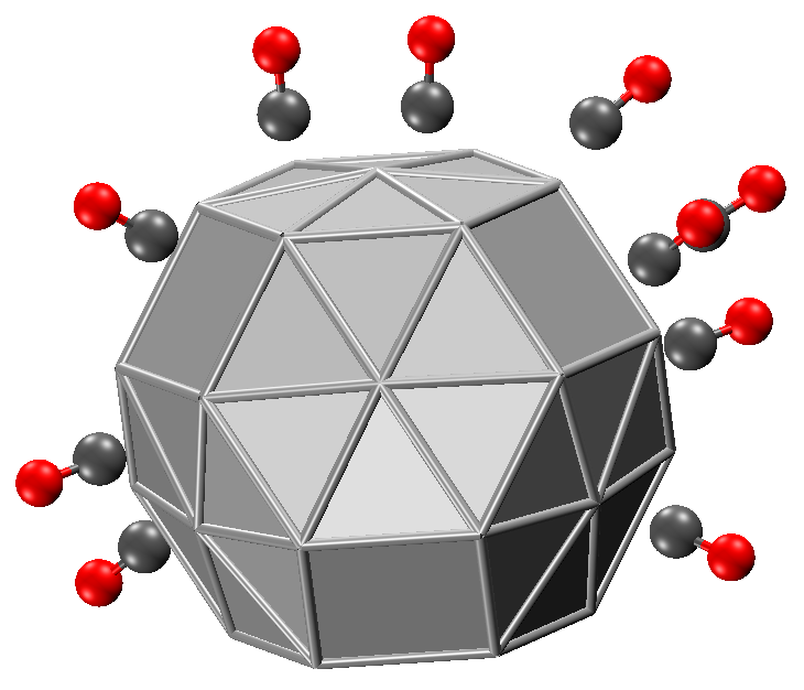
6.3.6. Example: absorb, (CO)10@Ag38

There is a very useful keyword absorb in geom: with it you can put molecules on the surface of a molecule, like a metal slab or protein.

Note

absorb n1 n2 n3

Randomly distribute molecules on the surface of component n1 (index starting from 1). These molecules take a direction that the vector from atom n2 to n3 points along the local normal.

Let’s show this with an example. Consider 10 \(\text{CO}\) absorbed on \(\text{Ag}_{38}\). The structures of \(\text{Ag}_{38}\) and \(\text{CO}\) are given below:

ag38.xyz

38
Ag38
Ag        1.83581324854909   -0.66521416103382   -4.05084800386537
Ag        3.26146602865993    1.43076353307629   -2.74559379561526
Ag       -1.86766331981303   -3.69246865502893    1.76047772000301
Ag       -1.83581102159633    0.66521241553523    4.05084656236035
Ag       -4.37635842854696    0.46053090761453    0.92628644673458
Ag        0.15602085746999    2.00172223612582   -0.25803332624779
Ag        4.09045041549422   -0.07826673249061    1.86662431725502
Ag        2.96684423722295   -2.41279942319018    0.63392161141815
Ag        1.27537017794612    0.10273478583599    1.56858140117429
Ag        0.49180992899154    1.78611199051730   -3.40510826327950
Ag       -1.27542752460590   -0.10273282991459   -1.56852780260341
Ag        1.86765806332299    3.69248093139238   -1.76047676908242
Ag        1.58003106702717    4.07712387902652    1.04989147026445
Ag        1.24797585452742   -4.25706785477554   -0.73581396857223
Ag       -0.97472878274367   -0.48635742691014   -4.36290889209247
Ag        1.56411023996142   -0.28340514372109   -1.25313947728674
Ag       -3.31177359770293   -2.01320436495574   -0.06340730066674
Ag        0.96033695393650   -3.87241791982209    2.07453413622748
Ag       -0.49179643241507   -1.78609168703799    3.40506272467468
Ag        0.97471867683167    0.48635633328589    4.36290696130676
Ag        4.37636506050101   -0.46053366775522   -0.92629395693753
Ag        2.95063571629445   -2.55651271910380   -2.23163152893035
Ag       -1.24798342397203    4.25705941555808    0.73581747916760
Ag       -2.37713910520774    1.78950388800175   -3.37174214960943
Ag        2.37713234562125   -1.78950289396663    3.37174836642454
Ag        3.31183702084341    2.01323876759066    0.06340286526436
Ag       -0.96034478186356    3.87241695907278   -2.07452887108150
Ag       -3.26146124524853   -1.43076585076549    2.74558710274998
Ag       -2.95063365988223    2.55651250079272    2.23162668919665
Ag       -1.58003774094824   -4.07711813992677   -1.04988736473955
Ag       -2.68795036663320   -2.19763079149194   -2.85783568469868
Ag       -4.09044728739259    0.07826707984227   -1.86660956451639
Ag       -0.14676607800026    2.64016188401185    2.83464031184915
Ag        0.14677416984600   -2.64018472712655   -2.83466944323257
Ag       -0.15608921802641   -2.00170980842979    0.25806971579687
Ag        2.68794654621046    2.19763200878331    2.85784466194340
Ag       -2.96679571349412    2.41276479806487   -0.63391785806270
Ag       -1.56408890116479    0.28339049331867    1.25310346730934

co.xyz

2
CO
C         0.00000000000000    0.00000000000000   -0.06362328061977
O         0.00000000000000    0.00000000000000    1.06362328061977

Now we prepare the input:

ag38-co10.inp

lm_dir  ag38-co10
components
    ag38.xyz 1
    fix 0 0 0 0 0 0
    ****
    co.xyz 10
    absorb 1 1 2
    ****
end

First, we simply fix \(\text{Ag}_{38}\) as (0, 0, 0) without rotations, then let 10 \(\text{CO}\) absorb on the 1``st component, with the vector formed by the ``1``st and ``2``nd atom of ``co.xyz pointing outward. Let’s run the optimization:

Run the program:

$ geom ag38-co10.inp > ag38-co10.out

Let’s check out a structure, say ag38-co10/3.xyz, which is shown below.

If you change absorb 1 1 2 to absorb 1 2 1, you will see that oxygen atoms of \(\text{CO}\) will contact with the metal slab surface.

6.3.7. Example: shell, (CH3CN)10

Note

shell n1 n2 x y z a b c

Uniformly distribute molecules over an ellipsoid centered at (x, y, z) with 3 radii a, b, and c. These molecules take a direction that the vector from atom n1 to n2 points along the local normal.

shell n1 n2 n3 n4 x y z a b c

Uniformly distribute molecules over an ellipsoid centered at (x, y, z) with 3 radii a, b, and c. These molecules take a direction that the vector from the center of n1, n2 to the center of n3, n4 points along the local normal.

shell n1 n2 n3 n4 n5 n6 x y z a b c

Uniformly distribute molecules over an ellipsoid centered at (x, y, z) with 3 radii a, b, and c. These molecules take a direction that the vector from the center of n1, n2, n3 to the center of n4, n5, n6 points along the local normal.

shell is a powerful keyword in geom which enables you to build:

Micelle, anti-micelle structures;

Ligated clusters.

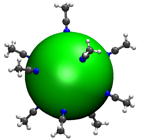
These two applications will be discussed in this and following sections. In this section, we will show how to let 10 \(\text{CH}_3\text{CN}\) uniformly distribute over a sphere.

The structure of \(\text{CH}_3\text{CN}\) is given below:

ch3cn.xyz

6
CH3CN
C                  0.00000000    0.00000000   -1.22619100
H                  0.00000000    1.00880600   -1.58285700
H                 -0.87365100   -0.50440300   -1.58285700
H                  0.87365100   -0.50440300   -1.58285700
C                  0.00000000    0.00000000    0.31380900
N                  0.00000000    0.00000000    1.46040900

Use the following input:

ch3cn10.inp

lm_dir  ch3cn10
components
    ch3cn.xyz 10
    shell 6 5 0 0 0 5 5 5
    # Or you can use the following:
    # shell 6 6 6 2 3 4 0 0 0 5 5 5
    ****
end

Here, 0 0 0 5 5 5 means that molecules will be distributed over the ellipsoid centered at (0, 0, 0) with 3 radii 5, 5, 5 (so it is a sphere). In the first way, 6 5 means that atom 6 is closer to the ellipsoid, and 6 5 points along the local normal; in the second way, 6 6 6 2 3 4 means that the center of atom 6 6 6 (i.e. the nitrogen atom) is closer to the ellipsoid, and the center of 2 3 4 (i.e. the three hydrogen atoms) is pointing outwardly. The two ways have the same effect.

Run the program:

$ geom ch3cn10.inp > ch3cn10.out

Let’s check out a structure, say ch3cn10/6.xyz, which is shown below.

6.3.8. Example: layer, (C4H2)30

layer can let molecules for a layer. This is very useful for building films, membranes, etc.

Note

layer n1 n2 n3 x0 y0 z0 x1 y1 z1 x2 y2 z2 x3 y 3 z 4

A finite layer is determined by 3 points: (x1, y1, z1), (x2, y2, z2), and (x3, y3, z3). Molecules will be distributed on the plane with a direction that the vector from atom n2 to n3 points along the local normal (x0, y0, z0). If n1 is 1, molecules will be distributed regularly; if it is 2, then distributed randomly.

For example, we want to arrange 30 \(\text{C}_4\text{H}_2\) to form a 5x5x5 film. The structure of \(\text{C}_4\text{H}_2\) is:

c4h2.xyz

6
C4H2
C                 -0.00000000   -0.00000000   -1.97120000
H                 -0.00000000   -0.00000000   -3.04120000
C                 -0.00000000   -0.00000000   -0.77000000
C                  0.00000000   -0.00000000    0.77000000
C                  0.00000000   -0.00000000    1.97120000
H                  0.00000000   -0.00000000    3.04120000

This is a linear molecule. The following input can be used:

c4h230.inp

lm_dir  c4h230
components
    c4h2.xyz 30
    layer 1 2 1 0 0 1 5 0 0 5 5 0 0 5 0
    ****
end

Here, 5 0 0 5 5 0 0 5 0 defines a layer of (5, 0, 0), (5, 5, 0), and (0, 5, 0). 2 1 means that atom 2 is closer to the layer, and 2 1 points along the local normal (0, 0, 1),. The first 1 means they are distributed regularly.

Run the program:

$ geom c4h230.inp > c4h230.out

Let’s check out a structure, say c4h230/3.xyz, which is shown below.

You can try to see what you will get by changing 2 1 1 to 2 1 2.